“Why Should I Trust You?”: Explaining the Predictions of Any Classifier Ribeiro et. al, CoRR Mar 2016.

Trusting predictions

If the users do not trust a model or a prediction, they will not use it.

This paper focuses on explaining example predictions of any given classifier in order to build trust in individual predictions and in the model as a whole.

It is important to differentiate between two different (but related) definitions of trust: (1) trusting a prediction, i.e. whether a user trusts an individual prediction sufficiently to take some action based on it, and (2) trusting a model, i.e. whether the user trusts a model to behave in reasonable ways if deployed. Both are directly impacted by how much the human understands a model’s behaviour, as opposed to seeing it as a black box.

These explanations are intended to supplement traditional evaluation metrics such as accuracy on a test set, which are sometimes good for tuning a model but not sufficient for building trust with humans. The authors also note that training and test sets derived from the same underlying data set often share biases, so that cross-validated models perform better in test than they do in the real world.

Explanations

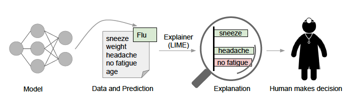
Explanations as used here are textual or visual artifacts illustrating how an instance’s attributes relate to the model’s prediction.

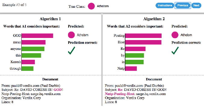
In addition to providing confidence in individual predictions or in the model as a whole, these example-based explanations can help practitioners in model selection and feature engineering. This essentially helps humans apply their domain knowledge to these tasks. In the following example, while algorithm #2 had a higher measured accuracy, algorithm #1 is clearly basing it’s prediction on more relevant features.

LIME – Local, Interpretable, Model-agnostic Explanations

The goal is to provide explanations that are

• Locally-faithful – correspond to how the model behaves in the vicinity of a given instance
• Interpretable – provide explanations that accommodate human limitations, e.g. involving a small number of simple properties
• Model-agnostic – able to explain any type of classifier

The LIME method creates an explanation for an individual prediction by building a simple interpretable model that reflects the behavior of the complex global model in the local vicinity of the example.

An interpretable representation is a point in a space whose dimensions can be interpreted by a human. Practically speaking, this paper uses small binary vectors of simple features. For instance, a text classifier might use a large space of word embeddings and ngrams as its input representation, while the explanation would use the presence or absence of a handful of particular words as an interpretable representation. The paper specifically focuses on finding sparse linear models as explanations, but notes that the same technique could be used to generate decision trees or falling rule lists as interpretable models. All of these are assumed to be over a domain \( \{0,1\}^{d’} \) of interpretable components – i.e. a reasonably small number of human interpretable features.

LIME frames the search for an interpretable explanation as an optimization problem. Given a set \({G}\) of potentially interpretable models, we need a measure \( \mathcal{L}(f,g,x) \) of how poorly the interpretable model \( g \in G \) approximates the original model \(f\) for point \(x\) – this is the loss function. We also need some measure \( \Omega(g) \) of the complexity of the model (e.g. the depth of a decision tree). We then pick a model which minimizes both of these

\[ \xi(x) = argmin_{g \in G} \mathcal{L}(f,g,x) + \Omega(g) \]

LIME algorithm

For a given example in the original input space \( x \in R^d \), we want to learn a locally faithful linear model in a relatively small feature space. The intuition is shown in the following diagram.

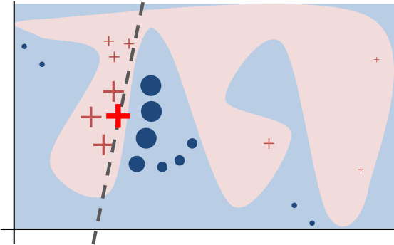
The bold red cross represents the instance being explained. The pink blob in the background represents the complex model \( f \). The dashed line is the learned linear model \( g \) which will be used as an explanation. This function is locally faithful to \( f \) but globally does not behave at all similarly.

The general approach is to search for the optimal explanatory model \( g(x) \) by sampling in the vecinity of the example x. We then search the space of potential explanatory models for one which optimizes the objective function \( \mathcal{L} + \Omega \).

The paper focuses on a couple concrete implementations of this approach. For text classification, the interpretable representation is a bag of words of maximum size \( K \). For image recognition, the interpretable representation is a binary vector of “super-pixels” of maximum size \( K \). The K features are selected first, using a regression technique, and then the weights of the linear model \( g \) are selected using a least-squares regression, weighted by the distance between the sample \( z \) and the original point \( x \).

• Starting from a point \(x\) in the original input space map it to a corresponding point \(x’ \in \{0,1\}^{d’} \) in the interpretable space.
• Then take random samples \( z’ \) around \( x’ \)
• Map each sample \(z’\) back to a point \(z\) in the original space and get the prediction \( f(z) \) using the original global model.
• Calculate the distance \( \Pi_x(z) \) between the sample point and the original point
• Fit the weights of \(g\) to minimize the error \(f(z) - g(z’)\) between the explanatory model and the global model for the set of perturbed examples, weighted by the distance of the perturbed example from the original example.

This process learns a linear function that closely matches the global function in the vicinity around \(x\).

Image recognition example

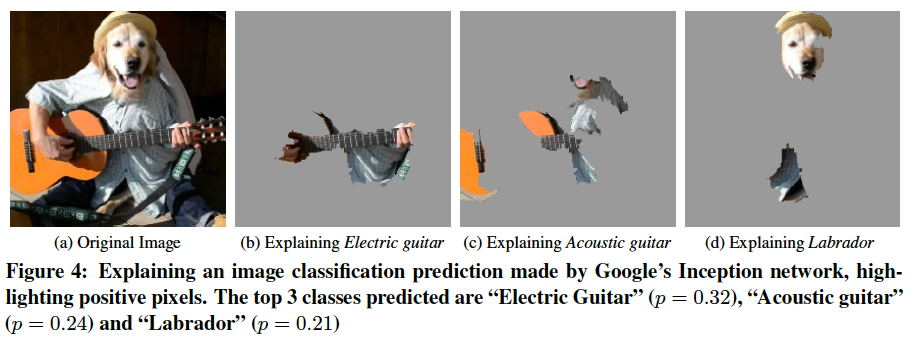
The paper gives an intriguing example of explaining the top 3 classes predicted by Google’s Inception neural network on an arbitrary image. For each of the top predicted classes, an explanation is produced by learning a linear model for each super-pixel in the image. (A super-pixel is a region of the image produced by a standard image segmentation algorithm). Then the super-pixels having the highest positive weight towards the predicted class are shown, with the negative super-pixels greyed out. This essentially allows the human observer to visualize some of the most pertinent regions of a very complex decision boundary.

Explaining models

The paper goes on to describe a technique for selecting a set of examples that will serve well for human evaluation of the model as a whole. The intuition here is to pick a reasonably small set of examples that cover the set of interpretable features as well as possible, with a bias towards the most explanatory features. Since the problem of maximizing a weighted coverage function is known to be NP-hard, a greedy algorithm is used to approximate the optimization function.

Validation

The paper goes on to justify the effectiveness and utility of the LIME method via simulation and human testing. The results show that, using such explanations, non-expert users are able to pick the classifier that generalizes better, even when the best classifier has worse accuracy when measured against the a test set. They are also able to effectively able to tune a model through feature selection when guided by such explanations, by removing features that they deem unimportant.

Conclusion

This paper presents a very compelling paradigm for producing example-based explanations of complex classifiers which can truly be useful in building trust in specific predictions and in selecting and tuning models without deep ML expertise. I have worked on several projects in the past which eschewed advanced ML algorithms due to the need for explainability. The type of technique explored here point towards a path where we can utilize the power of complex predictive models while still providing useful explanations.